This demo demonstrates how an regularized solutions can be computed using the toolbox.
It starts with the operator created by the demo bbdemo_deblur1, so please start with that.
To start it directly, use: playshow bbdemo_deblur3
The operator created in the first part of the demo is available in a separate script that does not produce graphical figures.
It also creates the inline-function IMGSHOW to display a non-negative image corrected for the gamma of the display.
bbdemo_deblurop;
Since this is an artifical example, our right-hand-side, B, of the equation system A*X=B will come from the known ground-truth, which is the masked test image.
For inverse systems, the "measurement" B is usually polluted by noise. In the simplest case the noise is an additive vector with independent elements of the same variance. If this is not the case, the system can be "pre-whitened" if the correlation is known or can be estimated.
The common case "weighted least-squares" refers to the situation where the elements are independent but needs to be scaled to have the same variance. This can be handled by solving the system W*A*X=W*B, where W=BBDIAG(1./STD) where STD is a vector with the standard deviation of each element.
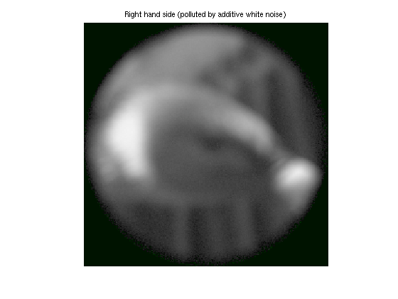
We demonstrate the simplest case of additive white noise. For specificity, we add two percent noise.
b=A*img1;
b=b+randn(size(b))*(.02*norm(b)/sqrt(length(b)));

clim=[0,max(img1(:))*1.1];
bbimagein(reshape(Mo'*b,dim3),clim);
axis image off;
title('Right hand side (polluted by additive white noise)');
As in the unregularized case, the hard work is performed by BBPRESOLVE. We need to inform it that we intend to compute regularized solutions.
Note: this may take several minutes even on a fast computer. Please keep in mind that the system is 43625-by-38024.
opt=struct('reg',true);
S=bbpresolve(A,b,opt);
xh=bbsolve(S);

bbimagein(reshape(Mi'*xh,dim1),clim);
axis image off;
title('Unregularized solution');
  Iteration: 5, residual: 6.9231e-02
  Iteration: 9, residual: 4.0151e-02
  Iteration: 13, residual: 3.2928e-02
  Iteration: 17, residual: 2.8470e-02
  Iteration: 21, residual: 2.5787e-02
  Iteration: 25, residual: 2.4354e-02
  Iteration: 29, residual: 2.3966e-02
Halting: max. number of iterations reached.
(Increase rmaxi or rkeep to improve the solution.)
Residual norm: 2.3925e-02 (resolved triplets only)
Residual norm: 8.5697e-03 (unregularized solution)
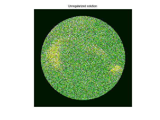
Clearly, the unregularized solution is a useless approximation of the original image.
Regularization balances the accuracy of a solution with amplification of noise. This balance is regulated by a "regularization parameter".
In the following we shall use Tikhonov-regularization, known as "ridge regression" by statisticians. (The toolbox allows any regularization method which can be formulated in terms of filter-factors.)
Selecting a suitable parameter can be difficult and may be subjective. Fortunately, it is quite fast to compute a number of regularized solutions after BBPRESOLVE is finished.
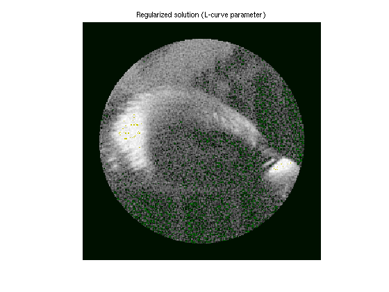
BBTools include a function which proposes a parameter based on the L-curve heuristic.
[lambda,LCurve]=bblcurve(A,S,'tikhonov');
xh=bbregsolve(S,'tikhonov',lambda);

bbimagein(reshape(Mi'*xh,dim1),clim);
axis image off;
title('Regularized solution (L-curve parameter)');
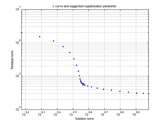
The L-curve method is a double-logarithmic plot of the norm of the residual and the solution. This usually have the shape of an L, hence the name of the method. It then estimates the position where the (signed) curvature is maximum, i.e. the corner of the L.
BBLCURVE computes these norms for a range of parameters, based on the singular values computed by BBPRESOLVE.
d=b-A*xh;

loglog(LCurve.xh_n,LCurve.res_n,'.'); hold on
loglog(norm(xh),norm(d),'sk'); hold off
title('L-curve and suggested regularization parameter');
xlabel('Solution norm'); ylabel('Residual norm');
grid on
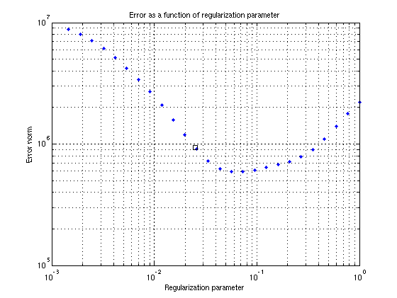
Since we are in the unusual situation that we know what we know what the solution should be (in the absence of noise), we may plot the difference between the ground truth and the regularized solution.
This shows that regularization is necessary. It also reveals that the L-curve method choose a somewhat underregularized solution.
l=length(LCurve.lambda);
err_n=zeros(l,1);
for i=1:l
  xhat=bbregsolve(S,'tikhonov',LCurve.lambda(i));
  err_n(i)=norm(img1-xhat);
end

loglog(LCurve.lambda,err_n,'.b'); hold on
loglog(lambda,norm(img1-xh),'sk'); hold off
title('Error as a function of regularization parameter');
xlabel('Regularization parameter');
ylabel('Error norm');
grid on;
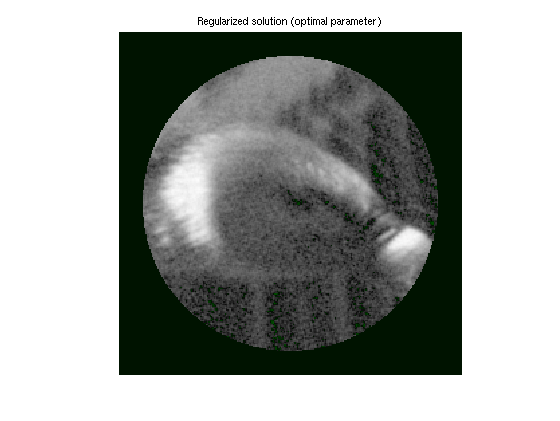
If we know a good best regularization parameter, we can get quite close to the original image. It should be emphasized that this is an "oracle solution" in the sense that the parameter used here is derived by knowing the solution.
It is, however, often possible to get close to such a solution by analyzing the solution for known properties, or (in the case of images) simply by inspection.
[empty,inx]=min(err_n);
lambda2=LCurve.lambda(inx);
xh2=bbregsolve(S,'tikhonov',lambda2);

bbimagein(reshape(Mi'*xh2,dim1),clim);
axis image off;
title('Regularized solution (optimal parameter)');