Tomography is the science of "slice drawing" (from Greek tomos+graphie). This demo is concerned with PET and SPECT widely used in medicin. Among other things, they are used to diagnose cancer, epilepsy, and Alzheimer's disease.
BBTools implements the two most common algorithms used to produce images: FBP (Filtered Back-Projection) and EM (Expectation Maximization). This demo shows how to use the FBP algorithm.
To start it directly, use: playshow bbdemo_tomo1
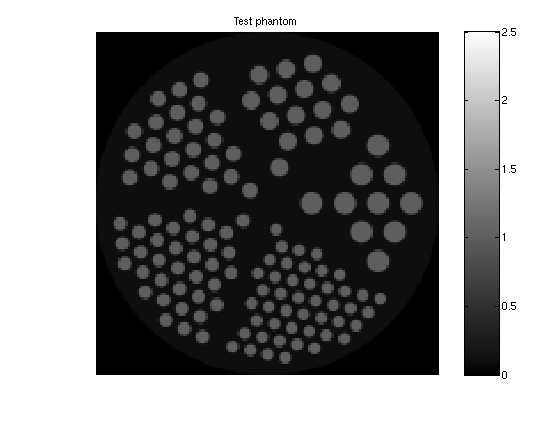
First we create a test-image so we have a goal target. In the current context, such an image is known as a phantom.
For PET and SPECT, the image represents concentrations of an injected radioactive substance. Therefore, the image is entirely positive.
We define the color-limits of the image for later comparison. We use BBIMAGEIN to compensate for the non-linear response of the display.
I_dim=[150,150];
img=bbphantom(I_dim,'restest',5,[],.1);

clim=[0,2.5];
bbimagein(img,clim,'l');
axis image off; colorbar;
title('Test phantom');
To understand the scanner, you may think of the volume as a semi-transparent gel. The scanner produces a set of images, plane projections, from a number of angles by rotating around the object.
Traditionally, we only see a single slice at a time, so each plane projection is just a line. This set of lines can be lined up side-by-side to form a so-called sinogram. This is known as a Radon transform.
To create the Radon transform, we need to tell how large the image is, what angles we are viewing it from, and (optionally) how densely we sample the projection plane.
Unlike the function RADON, found in the image processing toolbox from Mathworks, the Radon transform is created as an operator. To transform an image, it must be multiplied as shown next.
theta=(0:5:175);
[A,S_dim]=bbradon(size(img),theta);
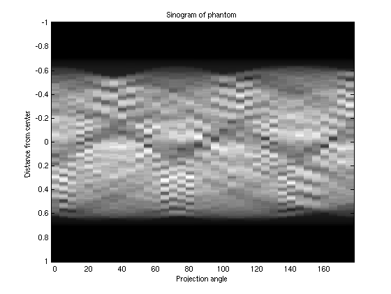
We get the sinogram by applying the Radon operator to the phantom image. We see clearly that the image is scrambled beyond recognition.
S=A*img(:);

dist=1-2*(0:S_dim(1)-1)/(S_dim(1)-1);
imagesc(theta,dist,reshape(S,S_dim));
colormap(gray);
title('Sinogram of phantom');
xlabel('Projection angle');
ylabel('Distance from center');
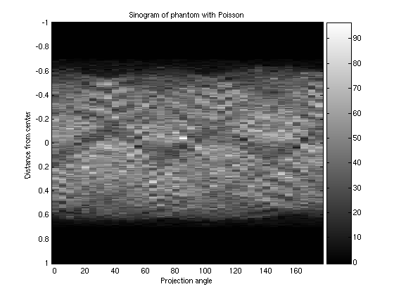
It would be nice if the sinogram above represented the data from the scanner. However, you are only allowed to inject a very small amount of radioactive substance into a human being. Usually, the radioactive dose is limited to roughly the level an air crew is exposed to on a year.
Since we are dealing with radioactive decay, the actual counts are governed by the Poisson distribution. Each element of the sinogram can be modeled roughly as independent random variables with the mean of the noise-less sinogram.
BBTools includes a function, BBRAND, which can do this. If you have the statistics toolbox from Mathworks, you could equally well use POISSRND.
S=bbrand('poisson',S);

S_max=max(S(:));
imagesc(theta,dist,reshape(S,S_dim),[-.5,S_max+.5]);
colormap(gray); colorbar;
title('Sinogram of phantom with Poisson');
xlabel('Projection angle');
ylabel('Distance from center');
The sinogram is not really useful in itself. We want an image, which we can get by inverting the transform. In tomography this step is known as reconstruction.
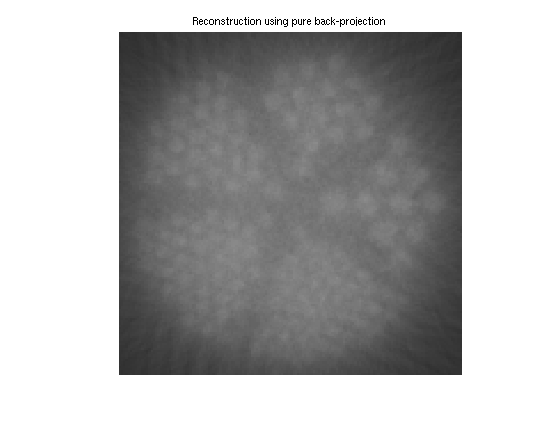
Filtered back projection is based on the idea of back projection. To see where the filtering comes into play, we first show what the reconstruction would look like if we simply used back projection.
This is easily accomplished in BBTools: the back-projection is the transpose (i.e. adjoint) of the Radon transform. However, we need to account for the fact that we have a number of projections, so we need to scale the image to get a direct comparison.
We see that the result is very blurry and generally inadequate for most uses.
img_bp=(A'*S)/(length(theta)^2);

bbimagein(reshape(img_bp,size(img)),clim,'l');
axis image off;
title('Reconstruction using pure back-projection');
We now apply the Filtered Back-Projection (FBP) method to reconstruct the original image. This was discovered shortly after the invention of the first scanner, and is still widely used.
The FBP method is a linear process, so in BBTools it is created as an operator. It assumes the sinogram represents angles equidistantly sampled from 0-180 degrees, so it only need the size of the sinogram as input.
[bb,dim]=bbfbp(S_dim);
img_fbp=bb*S;

bbimagein(reshape(img_fbp,dim),clim,'l');
axis image off;
title('Reconstruction using FBP');
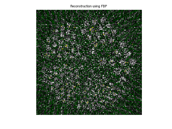
This image is unsatisfactory, because it amplifies the noise too much. The FBP-algorithm can compensate by filtering the response.
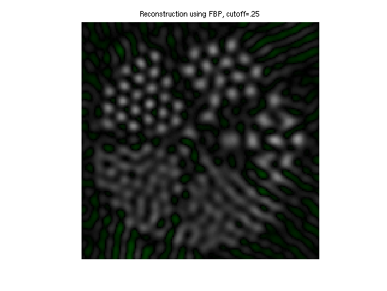
It is beyond the scope of this demo to explain filtering. It will suffice to explain that you may specify a cut-off frequency between 0 and 1, where 1 produce the most noisy image, which gets smoother as the cut-off approaches zero.
Note that smoothing comes at a loss of resolution. The ultimately smooth image (cut-off 0) is blank and contains no information.
[bb,dim]=bbfbp(S_dim,'cut',.25);
img_fbp=bb*S;

bbimagein(reshape(img_fbp,dim),clim,'l');
axis image off;
title('Reconstruction using FBP, cutoff=.25');
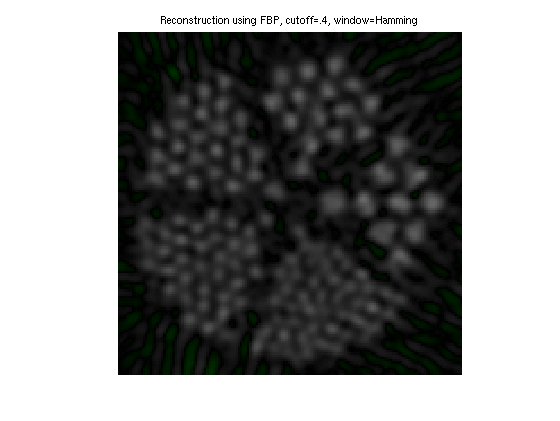
Another artifact often seen in reconstructed images, is called "ringing". In this context is usually manifest itself as "streak artifacts". You may, for example, see this as lines radiating from the center and outwards. The term comes from electronics and is meant in the sense of a bell-ringing.
To reduce this kind of artifacts, it is common to modify the filter using a window. It may be confusing, because it is considered a sport in signal processing to invent new windows, so there are plenty to choose from.
In pratical terms, the most important difference is whether you apply a window on top of the filter or not. We shall stick to the Hamming window below. Also, if we apply a window, we can often increase the cut-off frequency.
[bb,dim]=bbfbp(S_dim,'cut',.4,'hamming');
img_fbp=bb*S;

bbimagein(reshape(img_fbp,dim),clim,'l');
axis image off;
title('Reconstruction using FBP, cutoff=.4, window=Hamming');